UTM building in Excel or Google sheets

UTM building is probably not something your Ad operations team enjoys doing. They need to get the ad copy right, the creatives ready after collaborating with multiple other teams, the pitches just right, and also publish the campaigns on time.

In the middle of all this creative and interesting work, lies the bothersome UTM parameters, which need to be appended to all the links that go out on all your campaigns.

The UTM building drudgery

Let’s accept it, it’s boring work that nobody really wants to do.

If you are using a UTM builder like Google’s Campaign URL builder, you will need to copy the Website URL each time, and add fields like source, medium, name, term and content multiple times, WITHOUT TYPOS AND ERRORS.

When you are doing hundreds of campaigns each month, as most organizations do today, this becomes a massive PAIN.

So what’s the solution?

The easiest and most commonly used is Excel or Google sheets. With some simple formulae and functions, you can generate any number of URLs with different URL parameters.

Excel or Google sheets for UTM tagging

Here’s a step-by-step guide to using Excel or Google sheets to generate your UTM parameters.

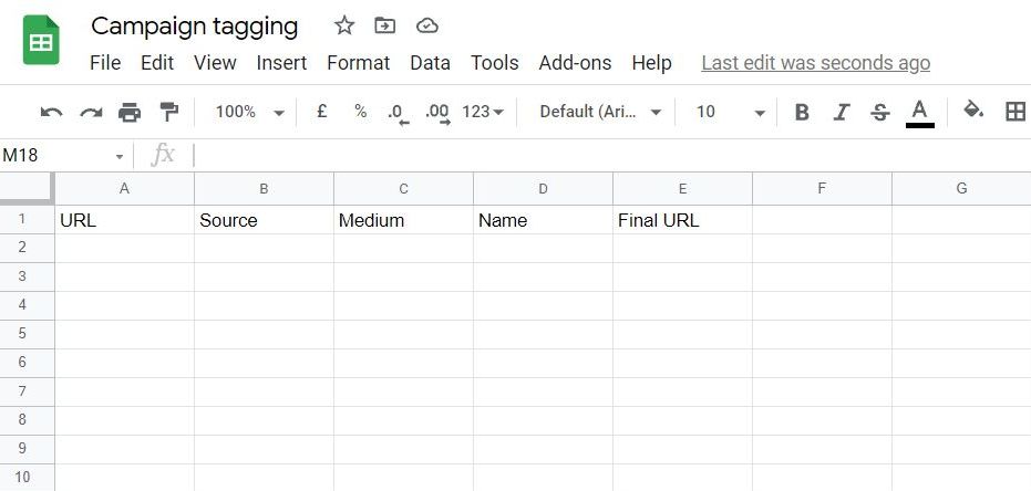
1. Go to Google sheets

2. Create a new spreadsheet

3. Enter the following in the top row – URL, Source, Medium, Name, Final URL

These are 3 basic parameters that are used for most URL tagging. But you are free to any number of parameters here.

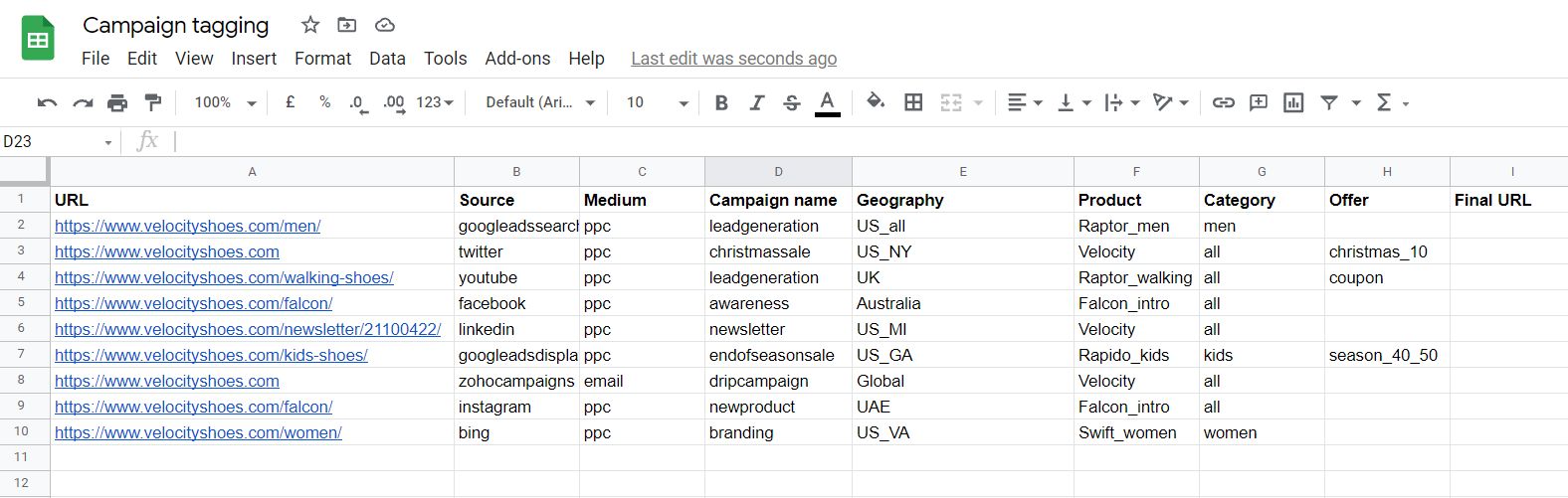
Let’s assume you are a Shoe seller called Velocity and you run campaigns through the year for different products.

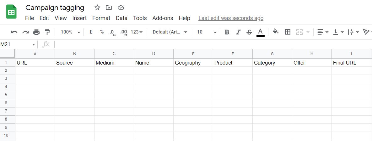
4. You can enter as many parameters or dimensions as you like, including terms like products, category, sub-category

Here I have added some key parameters that are important to a business like Velocity.

If you would like to know how to build standard UTM parameters, refer to our article on Basics of UTM parameters.

5. Start populating your sheet with data pertinent to your campaigns

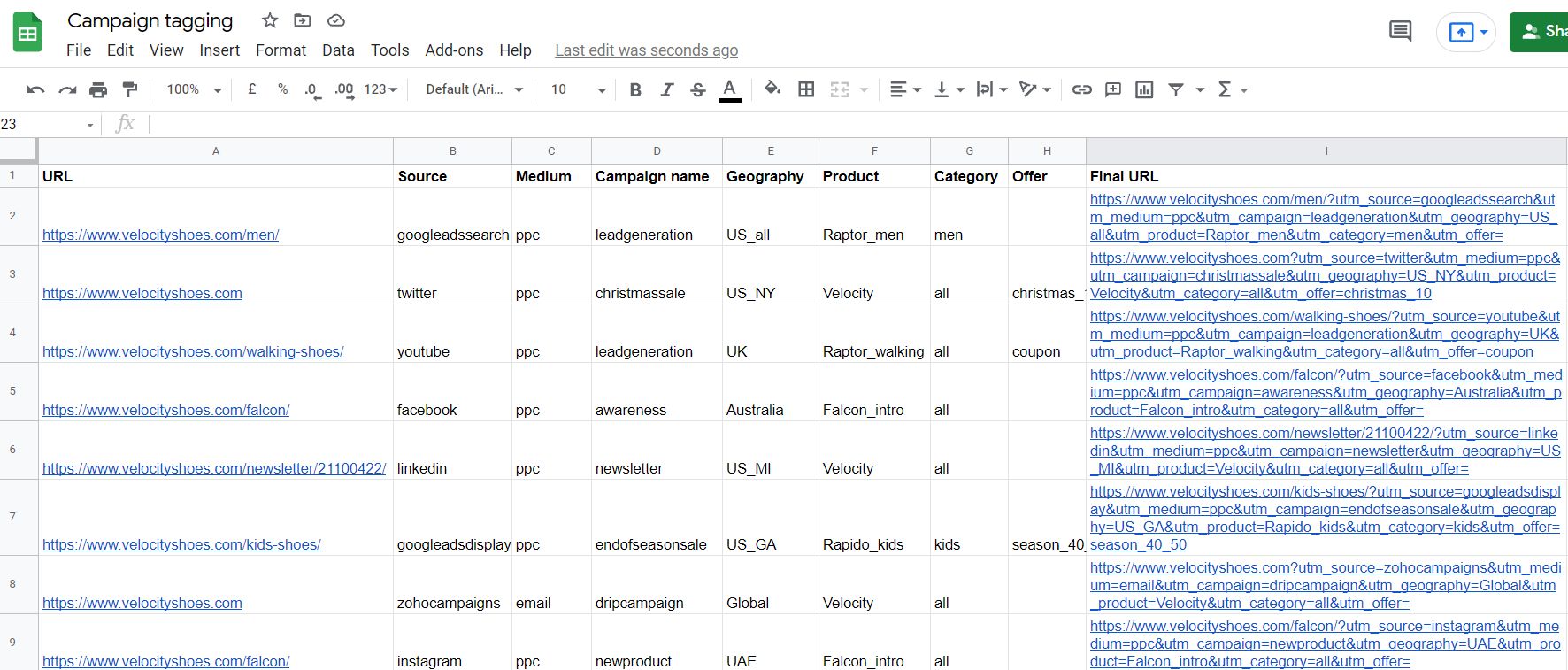
6. Concatenate formula in excel

Add this formula to the final column to combine the values in all the columns.

=CONCATENATE(A2,"?utm_source=",B2,"&utm_medium=",C2,"&utm_campaign=",D2,"&utm_geography=",E2,"&utm_product=",F2,"&utm_category=",G2,"&utm_offer=",H2)

This is a simple Concatenate function which can be made simpler or more complicated depending on the number of dimensions you have.

You would see the Final URL in this format below after you enter the formulae.

7. Data validation

This is a key step in your URL building. If your AdOps team adds their own versions of values to the Google sheet, you will end up with typos, data inconsistencies and a complete mess.

Data validation helps you define the superset of values you can have in any field.

1. Select the column you want, right click and go to Data Validation

   You could also go to the Data option on Toolbar and select Data Validation.

   The data validation screen pops up.

   
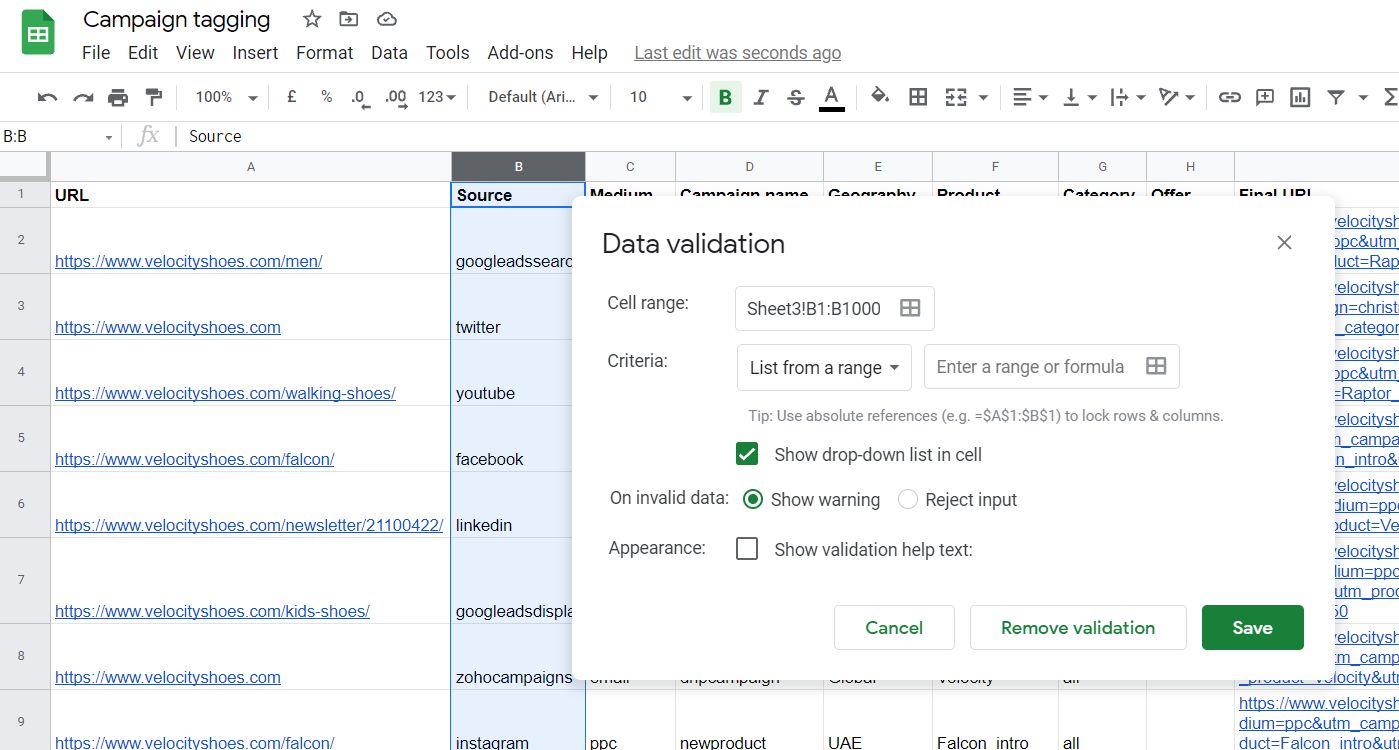
2. You have the option to select values for validation from a list, or to give a list of numbers, text, date, custom formulae etc. Here I am choosing List from a range.

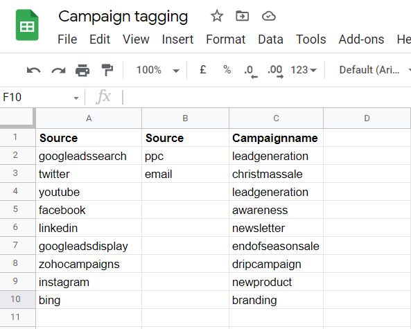
3. And for that, you need to create a list of values that can be added in a certain dimension. I am creating the list of values in the second sheet.

   

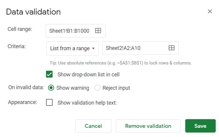
4. Once you have entered the superset of values you want, go back to the Data validation box, and click on the small table next to ‘Enter a range or formula’.

   Your data validation box should look like this.

   

5. Once you save, your Google sheet is ready to validate the values in each column. You can choose to Show warning or to Reject input completely. It is better to choose the Reject input option since that will prevent your team members from choosing other options.

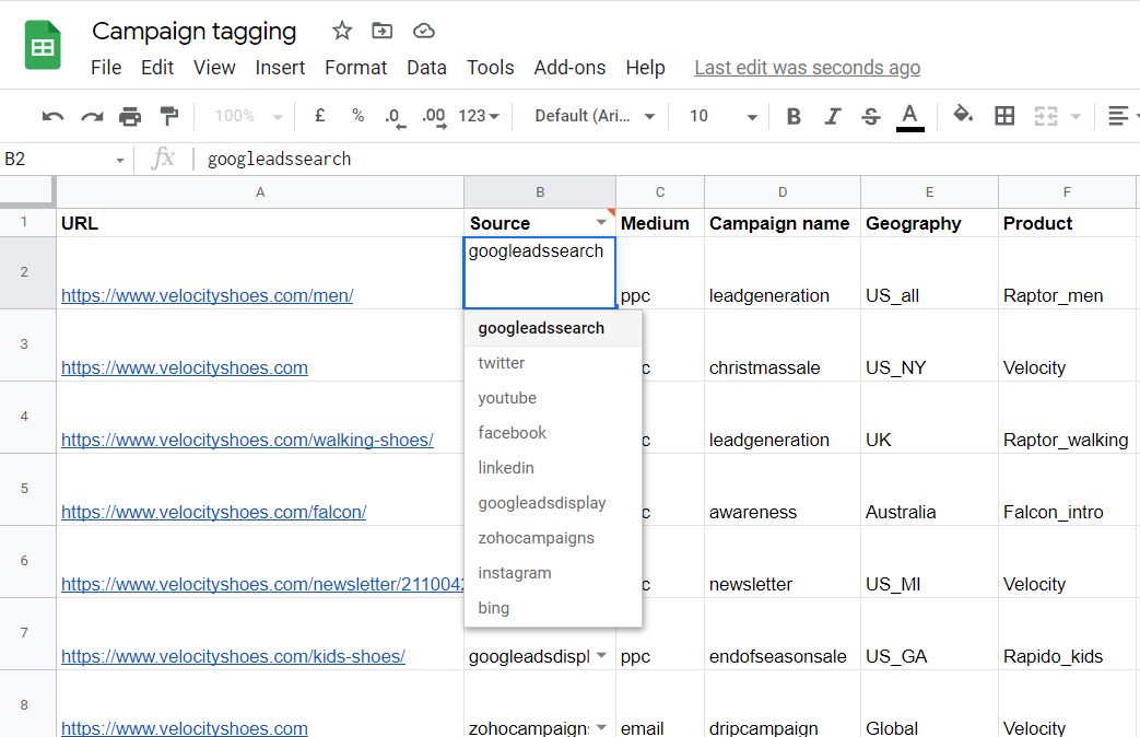
   While populating the sheet, values would have to be selected from the drop-down, and cannot be entered manually.

   

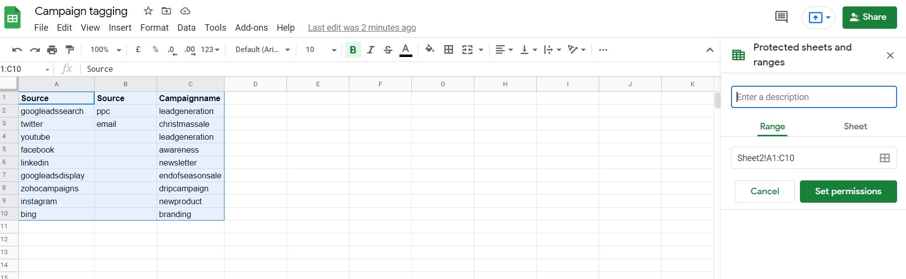
8. Lock data validation values

Google sheets would have to be to be shared between members who are creating campaigns, and this would result in errors, even if you specify data validation values. Make sure you lock the second sheet with values for dimensions specified.

Select the range of cells you want to lock, right click and go to ‘Protect range’. You can set permission for members who can edit this range of values, so that data integrity is maintained.

9. If-else statements

If you look at the final formula, you will see ‘utm_offer=’ at the end, without any value associated with it.

This happens when you have cells that are blank with no values.

Formula:

=CONCATENATE(A2,"?utm_source=",B2,"&utm_medium=",C2,"&utm_campaign=",D2,"&utm_geography=",E2,"&utm_product=",F2,"&utm_category=",G2,"&utm_offer=",H2)

Result:

https://www.velocityshoes.com?utm_source=googleadssearch&utm_medium=ppc&utm_campaign=leadgeneration&utm_geography=US_all&utm_product=Raptor_men&utm_category=men&utm_offer=

In these cases, you need to add a condition so that the dimension name and the value will not be added to the URL. Here’s the formula.

Formula:

=CONCATENATE(A2,"?utm_source=",B2,"&utm_medium=",C2,"&utm_campaign=",D2,"&utm_geography=",E2,"&utm_product=",F2,"&utm_category=",G2,if(ISBLANK(H2),,CONCATENATE("utm_offer=",H2)))

Result:

https://www.velocityshoes.com?utm_source=googleadssearch&utm_medium=ppc&utm_campaign=leadgeneration&utm_geography=US_all&utm_product=Raptor_men&utm_category=men

This takes care of the blank cells. I have added the ‘If-blank’ condition only for the last column H, so that the formula is not very confusing. But it can be used in all columns to ensure that blank cells are taken care of.

Advantages and Disadvantages of using Google sheets to create UTM tagging codes

Advantages:

1. Free software
2. Easy to access and use
3. Simple functionalities
4. Teams can collaborate to build the final sheet

Disadvantages:

1. Any of the users with ‘edit’ access can change columns or values in your main sheet resulting in errors, and data inconsistencies.
2. There is no easy way to handle dependecies between your UTM parameters. For example: A Facebook campaign UTM would not have email as its utm_source value.
3. If your campaigns are run by different teams, access permissions would have to be given for the complete sheet, and not for specific campaigns.

Try out CampTag – The awesome marketing taxonomy and URL builder

Camptag offers all the functionalities of Google sheets, and it also takes care of the disadvantages mentioned above. Take a free trial of our tool to see how you can get better data and returns on your marketing campaigns.

Contact Camptag now! Or would you like a free trial?